Probability Calculator

Probability of Two Events

To find out the union, intersection, and other related probabilities of two independent events.

Probability of A: P(A)
Probability of B: P(B)

Probability Solver for Two Events

Please provide any 2 values below to calculate the rest probabilities of two independent events.

Probability of A: P(A)
Probability of B: P(B)
Probability of A NOT occuring: P(A')
Probability of B NOT occuring: P(B')
Probability of A and B both occuring: P(A∩B)
Probability that A or B or both occur: P(A∪B)
Probability that A or B occurs but NOT both: P(AΔB)
Probability of neither A nor B occuring: P((A∪B)')

Probability of a Series of Independent Events

	Probability	Repeat Times
Event A
Event B

Probability of a Normal Distribution

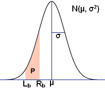
Use the calculator below to find the area P shown in the normal distribution, as well as the confidence intervals for a range of confidence levels.

Mean: (µ)
Standard Deviation (σ):
Left Bound (Lb):		For negative infinite, use -inf
Right Bound (Rb):		For positive infinite, use inf

Related

Standard Deviation Calculator | Sample Size Calculator | Statistics Calculator

Probability of Two Events

Probability quantifies how likely an outcome is, expressed as a value between 0 (impossible) and 1 (certain). In general it is the ratio of favorable results to all possible results, with considerations for independence, exclusivity, or conditioning. The tool below can calculate the chance that neither A nor B happens, the chance that A or B (or both) happen when they are not exclusive, the joint chance of A and B together, and the chance that exactly one of A or B occurs.

Complement of A and B

Given a probability A, denoted by P(A), it is simple to calculate the complement, or the probability that the event described by P(A) does not occur, P(A'). If, for example, P(A) = 0.65 represents the probability that Bob does not do his homework, his teacher Sally can predict the probability that Bob does his homework as follows:

P(A') = 1 - P(A) = 1 - 0.65 = 0.35

In this example Bob has a 35 % probability of completing his homework. The complement P(B') is obtained the same way. Note that the calculator assumes independence, so even when P(A) = 0.65, P(B) need not be 0.35; it could be 0.30 or any other value.

Intersection of A and B

The overlap of events A and B, denoted P(A \u2229 B) or P(A AND B), represents their combined likelihood (see Venn diagram). If A and B cannot occur together, then P(A \u2229 B) = 0—for example, rolling a 4 and a 6 on a single die is impossible, making the events mutually exclusive. When the events are independent, P(A \u2229 B) equals the product of their individual probabilities. For instance, the chance that two consecutive die rolls both show a six is calculated this way.

P(A ∩ B) = P(A) × P(B)

The calculator above assumes independent probabilities. When events influence each other we use conditional probability, written as P(A|B), the chance of A after B has occurred. Imagine a jar with 10 marbles—7 black and 3 blue. What is the probability of picking a black marble after a blue one has been removed without replacement (the jar now contains 9 marbles)?

1 6

×

1 6

= 0.0278

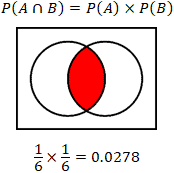
The calculator provided considers the case where the probabilities are independent. Calculating the probability is slightly more involved when the events are dependent, and involves an understanding of conditional probability, or the probability of event A given that event B has occurred, P(A|B). Take the example of a bag of 10 marbles, 7 of which are black, and 3 of which are blue. Calculate the probability of drawing a black marble if a blue marble has been withdrawn without replacement (the blue marble is removed from the bag, reducing the total number of marbles in the bag):

Probability of drawing a blue marble:

P(A) = 3/10

Probability of drawing a black marble:

P(B) = 7/10

Probability of drawing a black marble given that a blue marble was drawn:

This demonstrates that the odds of drawing a black marble depend on earlier draws made without replacement. Consequently, to find the probability of first pulling a blue marble and then a black one from the same container, we must account for the changed composition after the first draw.

As can be seen, the probability that a black marble is drawn is affected by any previous event where a black or blue marble was drawn without replacement. Thus, if a person wanted to determine the probability of withdrawing a blue and then black marble from the bag:

Probability of drawing a blue and then black marble using the probabilities calculated above:

In probability, the union of events, denoted P(A U B) (also written as P(A OR B)), refers to the chance that either one or both events occur (see Venn diagram). This is an inclusive OR: at least one event happens, and they may happen together. Unions fall into two categories: mutually exclusive events or events that are not mutually exclusive. When the events cannot occur together, the calculation simplifies:

Union of A and B

In probability, the union of events, P(A U B), essentially involves the condition where any or all of the events being considered occur, shown in the Venn diagram below. Note that P(A U B) can also be written as P(A OR B). In this case, the "inclusive OR" is being used. This means that while at least one of the conditions within the union must hold true, all conditions can be simultaneously true. There are two cases for the union of events; the events are either mutually exclusive, or the events are not mutually exclusive. In the case where the events are mutually exclusive, the calculation of the probability is simpler:

Take a standard six‑sided die. Let event A be “the roll is even” and event B be “the roll is odd.” These outcomes are mutually exclusive because a single roll cannot be both even and odd. Hence P(A U B) = 3/6 + 3/6 = 1, covering all possible faces.

The tool also handles the scenario where events A and B can occur together. In that situation:

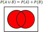
A basic example of mutually exclusive events would be the rolling of a dice, where event A is the probability that an even number is rolled, and event B is the probability that an odd number is rolled. It is clear in this case that the events are mutually exclusive since a number cannot be both even and odd, so P(A U B) would be 3/6 + 3/6 = 1, since a standard dice only has odd and even numbers.

Returning to the die, we want the probability that the result is either an even number or a multiple of three. The sample space consists of the six faces of the die, listed as:

The calculator can also compute P(A XOR B), illustrated in the Venn diagram below. The exclusive OR means that either A or B occurs, but never both at the same time. Its formula is:

Consider a Halloween scene where two candy bowls sit on the porch: one filled with Snickers, the other with Reese's. Bright signs tell each trick‑or‑treater to pick either a Snickers or a Reese's, but not both. Not every child follows the rule. If the chance of reaching for a Reese's is P(A) = 0.65 and the chance of reaching for a Snickers is P(B) = 0.349, and only P(unlikely) = 0.001 of kids actually resist the temptation to take both, compute the probability that exactly one of the two candies is selected:

	S = {1,2,3,4,5,6}
Probability of an even number:	P(A) = {2,4,6} = 3/6
Probability of a multiple of 3:	P(B) = {3,6} = 2/6
Intersection of A and B:	P(A ∩ B) = {6} = 1/6
	P(A U B) = 3/6 + 2/6 -1/6 = 2/3

Exclusive OR of A and B

Another possible scenario that the calculator above computes is P(A XOR B), shown in the Venn diagram below. The "Exclusive OR" operation is defined as the event that A or B occurs, but not simultaneously. The equation is as follows:

P(A XOR B) = P(A) + P(B) - 2 × P(A ∩ B)

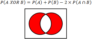
As an example, imagine it is Halloween, and two buckets of candy are set outside the house, one containing Snickers, and the other containing Reese's. Multiple flashing neon signs are placed around the buckets of candy insisting that each trick-or-treater only takes one Snickers OR Reese's but not both! It is unlikely, however, that every child adheres to the flashing neon signs. Given a probability of Reese's being chosen as P(A) = 0.65, or Snickers being chosen with P(B) = 0.349, and a P(unlikely) = 0.001 that a child exercises restraint while considering the detriments of a potential future cavity, calculate the probability that Snickers or Reese's is chosen, but not both:

Here μ denotes the mean and σ² the variance. The symbol σ, which also appears in the standard deviation calculator, stands for the standard deviation. When μ = 0 and σ = 1, the distribution becomes the standard normal distribution. The diagram above illustrates a typical bell‑shaped curve.

The normal (Gaussian) distribution is a handy model for any quantity that tends to cluster around a central value – for instance, male student heights, leaf dimensions, test scores, and so on. By using the \"Normal Distribution\" tool above you can find the likelihood that a normally‑distributed variable falls between two limits. For example, to estimate the probability that a university student’s height lies between 60 in and 72 in, given a mean of 68 in and a standard deviation of 4 in, first convert both limits to z‑scores (subtract the mean and divide by the standard deviation).

Normal Distribution

The normal distribution or Gaussian distribution is a continuous probability distribution that follows the function of:

The picture above highlights the region of interest under the normal curve. To turn that shaded area into a probability, consult the standard normal Z‑table at the bottom of the page. Several variants of Z‑tables exist; the one shown lists the area from the mean (0) up to a positive Z value. Other tables give the tail probabilities to the left or right, which can be combined by subtraction to obtain the desired area.

In this illustration, to find the probability between 0 and Z = 2, locate 2 in the left‑most column of the table – the table is designed to give the area from the mean (0) to the chosen Z. For Z = 2.11 you would read the entry where the row for 2.1 meets the column for 0.01, yielding 0.48257. Although the graph also shows negative Z values, the table only reports positive ones; because the normal curve is symmetric, the area from 0 to –2 equals the area from 0 to 2. Thus the probability from 0 to 2 is 0.47725, and from 0 to 1 it is 0.34134. Adding the areas for –2 to 0 and 0 to 1 gives 0.81859 (≈ 81.86 %). Hence a student has roughly an 81.9 % chance of being between 60 in and 72 in tall.

60 - 68 4

=

-8 4

= -2

72 - 68 4

=

4 4

= 1

The tool also generates tables of confidence intervals for a range of confidence levels. For a deeper dive, see the Sample Size Calculator for Proportions. In short, a confidence interval gives a range that likely contains the true population parameter rather than a single point estimate, and it is tied to a confidence level (often expressed as a percentage such as 95 %). The higher the level, the more reliable the interval is considered to be.

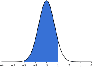
The graph above illustrates the area of interest in the normal distribution. In order to determine the probability represented by the shaded area of the graph, use the standard normal Z-table provided at the bottom of the page. Note that there are different types of standard normal Z-tables. The table below provides the probability that a statistic is between 0 and Z, where 0 is the mean in the standard normal distribution. There are also Z-tables that provide the probabilities left or right of Z, both of which can be used to calculate the desired probability by subtracting the relevant values.

For this example, to determine the probability of a value between 0 and 2, find 2 in the first column of the table, since this table by definition provides probabilities between the mean (which is 0 in the standard normal distribution) and the number of choices, in this case, 2. Note that since the value in question is 2.0, the table is read by lining up the 2 row with the 0 column, and reading the value therein. If, instead, the value in question were 2.11, the 2.1 row would be matched with the 0.01 column and the value would be 0.48257. Also, note that even though the actual value of interest is -2 on the graph, the table only provides positive values. Since the normal distribution is symmetrical, only the displacement is important, and a displacement of 0 to -2 or 0 to 2 is the same, and will have the same area under the curve. Thus, the probability of a value falling between 0 and 2 is 0.47725 , while a value between 0 and 1 has a probability of 0.34134. Since the desired area is between -2 and 1, the probabilities are added to yield 0.81859, or approximately 81.859%. Returning to the example, this means that there is an 81.859% chance in this case that a male student at the given university has a height between 60 and 72 inches.

The calculator also provides a table of confidence intervals for various confidence levels. Refer to the Sample Size Calculator for Proportions for a more detailed explanation of confidence intervals and levels. Briefly, a confidence interval is a way of estimating a population parameter that provides an interval of the parameter rather than a single value. A confidence interval is always qualified by a confidence level, usually expressed as a percentage such as 95%. It is an indicator of the reliability of the estimate.

	Search